OpenSeaMap-dev:En:Depth Data: Unterschied zwischen den Versionen
(→Meta Data Stats) |
Markus (Diskussion | Beiträge) K (Markus verschob die Seite Depth Data nach OpenSeaMap-dev:En:Depth Data: Entwickler-Seite von Jens) |
||
| (24 dazwischenliegende Versionen von 2 Benutzern werden nicht angezeigt) | |||
| Zeile 101: | Zeile 101: | ||
'''Vessel Metadata''' | '''Vessel Metadata''' | ||
{| class="wikitable" | {| class="wikitable" | ||
| + | |- | ||
| + | | VesselConfig ID || 68 | ||
|- | |- | ||
| Manufacturer || Bavaria Yachtbau | | Manufacturer || Bavaria Yachtbau | ||
| Zeile 118: | Zeile 120: | ||
| Sensor manufacturer || Raymarine | | Sensor manufacturer || Raymarine | ||
|- | |- | ||
| − | | Sensor Offset || 0,45 meters | + | | Sensor Offset to waterline || 0,45 meters |
| + | |- | ||
| + | | Sensor Offset to keel || 1,15 meters | ||
|} | |} | ||
| + | |||
| Zeile 144: | Zeile 149: | ||
The data in the dataset is not corrected by sensor offset. | The data in the dataset is not corrected by sensor offset. | ||
| − | === | + | ==== Baltic Sea Olpenitz (Germany)==== |
| + | |||
| + | In this test area we have tracks from two different vessel configurations. | ||
| + | The fist one was the one from the test area Großenbrode (config ID 68). | ||
| + | |||
| + | In the Table below the settings for die vesselconfigid 110 are shown: | ||
| + | |||
| + | '''Vessel Metadata''' | ||
| + | {| class="wikitable" | ||
| + | |- | ||
| + | | VesselConfigId || 110 | ||
| + | |- | ||
| + | | Manufacturer || Waarschip | ||
| + | |- | ||
| + | | Model || 570 | ||
| + | |- | ||
| + | | Length || 5,7 meters | ||
| + | |- | ||
| + | | Beam || 2,45 meters | ||
| + | |- | ||
| + | | Draft || 1,0 meters | ||
| + | |- | ||
| + | | Height || 9.1 meters | ||
| + | |- | ||
| + | | Displacement || 0,8 t | ||
| + | |- | ||
| + | | Sensor manufacturer || Tacktick/ Airmar | ||
| + | |- | ||
| + | | Sensor Model || T912 | ||
| + | |- | ||
| + | | Sensor Offset to waterline || 0,2 meters | ||
| + | |- | ||
| + | | Sensor Offset to keel || 0,45 meters | ||
| + | |} | ||
| + | |||
| + | [[Datei: Balitc_sea_scatter_plot_2.jpeg]] | ||
| + | |||
| + | [Picture 1] Scatterplot for vesselconfigID 110. Trendline in Black and optimal line in red (after correction of the sensor offset to waterline). | ||
| + | |||
| + | {| class="wikitable" | ||
| + | |- | ||
| + | | vsselConfigId || 110 | ||
| + | |- | ||
| + | | n || 247 | ||
| + | |- | ||
| + | | mean || 0,49 meters | ||
| + | |- | ||
| + | | rms || 0,62 meters | ||
| + | |- | ||
| + | | max|| 2,53 meters | ||
| + | |} | ||
| + | |||
| + | The distribution is quite different from the data recorded in the test area Großenbrode with an different sensor. | ||
| + | |||
| + | Fortunately we have also data from the VesselConfigId 68 in this test area to compare the measurements. | ||
| + | |||
| + | [[Datei: Balitc_sea_scatter_plot_2_68_all.jpeg]] | ||
| + | |||
| + | [Picture 2] Scatterplot for vesselconfigID 68 after correction of the sensor offset to waterline. | ||
| + | |||
| + | Obviously there are some outliers which are shown in picture 3. | ||
| + | |||
| + | [[Datei: Bsh 2 outliers.jpg]] | ||
| + | |||
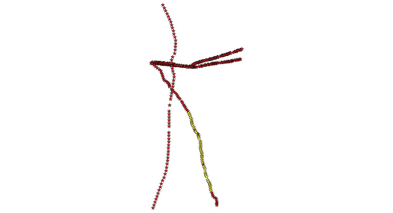
| + | [Picture 2] Outliers along the track 9064 in yellow - vesselconfigID 68. | ||
| − | + | Without the outliers the behavier of distribution is very same the results in the test area Großenbrode. | |
| + | |||
| + | [[Datei: Balitc_sea_scatter_plot_2_68_without.jpeg]] | ||
| + | |||
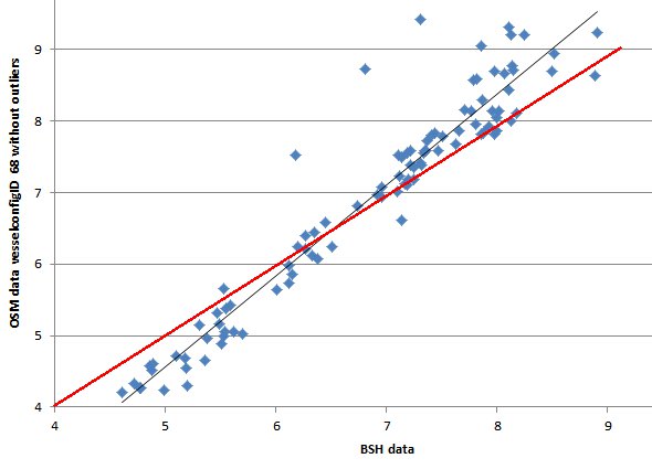
| + | [Picture 1] Scatterplot for vesselconfigID 68 without outliers. Trendline in Black and optimal line in red (after correction of the sensor offset to waterline). | ||
| + | |||
| + | {| class="wikitable" | ||
| + | |- | ||
| + | | vsselConfigId || 68 () without outliers | ||
| + | |- | ||
| + | | n || 100 | ||
| + | |- | ||
| + | | mean || 0,38 meters | ||
| + | |- | ||
| + | | rms || 0,53 meters | ||
| + | |- | ||
| + | | max|| 2,1 meters | ||
| + | |} | ||
| + | |||
| + | ==== Preliminary Conclusions ==== | ||
| + | |||
| + | 1. The distribution of the data derived from the measurements depends on the sensor. The realationships are almost linear and could be corrected if the sensor is known. Therefore the fill out in the form of the Web Frontend should be obligatory. | ||
| + | |||
| + | 2. The sensor offset to the waterline is very easy to correct and should be obligatory in the fill out in the form. | ||
| + | |||
| + | 3. There are outliers which should be investigated. Perhaps this data could be corrected or identified with the data from the uploaded tracks (speed, etc.). | ||
| + | |||
| + | === Meta Data Statistics === | ||
| + | |||
| + | Statistics for the metadata entrees with some personal comments (by MartinOver). Stand 20.9.2014. | ||
{| class="prettytable" | {| class="prettytable" | ||
| Zeile 759: | Zeile 857: | ||
* [http://users.isr.ist.utl.pt/~pedro/publications/CAMS10.pdf A Multiple Model Adaptive Wave Filter for Dynamic Ship Positioning] | * [http://users.isr.ist.utl.pt/~pedro/publications/CAMS10.pdf A Multiple Model Adaptive Wave Filter for Dynamic Ship Positioning] | ||
* [http://ieeexplore.ieee.org/xpl/login.jsp?tp=&arnumber=4449205&url=http%3A%2F%2Fieeexplore.ieee.org%2Fxpls%2Fabs_all.jsp%3Farnumber%3D4449205 Echosounder Depth Tracking with the Extended Kalman Filter] | * [http://ieeexplore.ieee.org/xpl/login.jsp?tp=&arnumber=4449205&url=http%3A%2F%2Fieeexplore.ieee.org%2Fxpls%2Fabs_all.jsp%3Farnumber%3D4449205 Echosounder Depth Tracking with the Extended Kalman Filter] | ||
| + | |||
| + | [[Kategorie:Depth-DB]] | ||
Aktuelle Version vom 29. Januar 2021, 15:05 Uhr
This Page describes the necessary efforts to retrieve and analyze depth data as well as create renderings from it
Inhaltsverzeichnis
Data Aquisition
Depth data can be retrieved from public domain sources or from crowd sourced data.
GEBCO
DIe Daten sind gerendert und stehen als Layer zur Verfügung:
| Zoom | Inhalt |
|---|---|
| 0..10 | Blaustufen und Schattierung |
| 11..18 | beschriftete Tiefenlinien, Blaustufen und Schattierung |
Noch zu lösende Probleme:
- der GEBCO-Layer erzeugt einen milchigen Schleier über der Basiskarte
- Tiefenlinien sind ab z=14 etwas grob (also ab da, wo dann die Flachwassertiefen beginnen) Karte
- Überschneidungen von 100m-Linie und Küstenlinie Karte
- Steilküsten (Cuba) Karte
Crowd Sourced Data
Crowd sourced data may be gathered by YOU. There are two options in development. A hardware and a software option.
Workflow
Here you can find the document with the previous thoughts about the workflow: PPT Dokument
Hardware logger
We are currently developing a hardware logger that may easily be plugged to the ship's network in order to log the networks data to a SD card. That data may then be uploaded by plugging the SD card to a normal computer with internet connection for upload. The main goal is to support NMEA 0183 data with options for NMEA 2000.
Software logger
A Software logger is in development and can be downloaded here.
It currently supports:
- Bluetooth
- Serial ports
- Internet Protocol (IP)
It processes NMEA 0183 and AIS data.
For vendor specific protocols such as SeaTalk 1 you have to use a converter to NMEA 0183 data.
NMEA 2000 support is only available if data is transcoded to NMEA 0183 by a converter.
Chart Plotters
Some chart plotters are able to save tracks out-of-the-box, e.g. several Raymarine (FSH files) and Humminbird (SON files) devices. Those files may directly be used as data source.
Upload Process
Uploading data is possible through using the OpenSeaMap Data Logger Software or via Web Interface. The system is currently being tested.
You'll find further information here.
Test Data
Brombachsee (Germany)
Test data for Openseamap: Brombachsee_Test_Data
dgm_brombachsee.tif: Digital Elevation Model of the sea derived from height lines WWA (C).
shapes_brombachsee.shp: Shape File derived from 4 NMEA Tracks. "dbs" is the original Sounding and "deep_cor" the depth after a correction (gauge levl).
gpx_brombachsee.gpx: ele = "dbs" from the Shape File
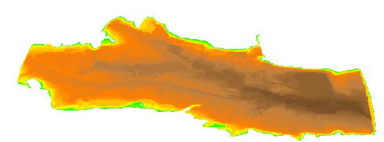 Resulting Digital Elevation Model
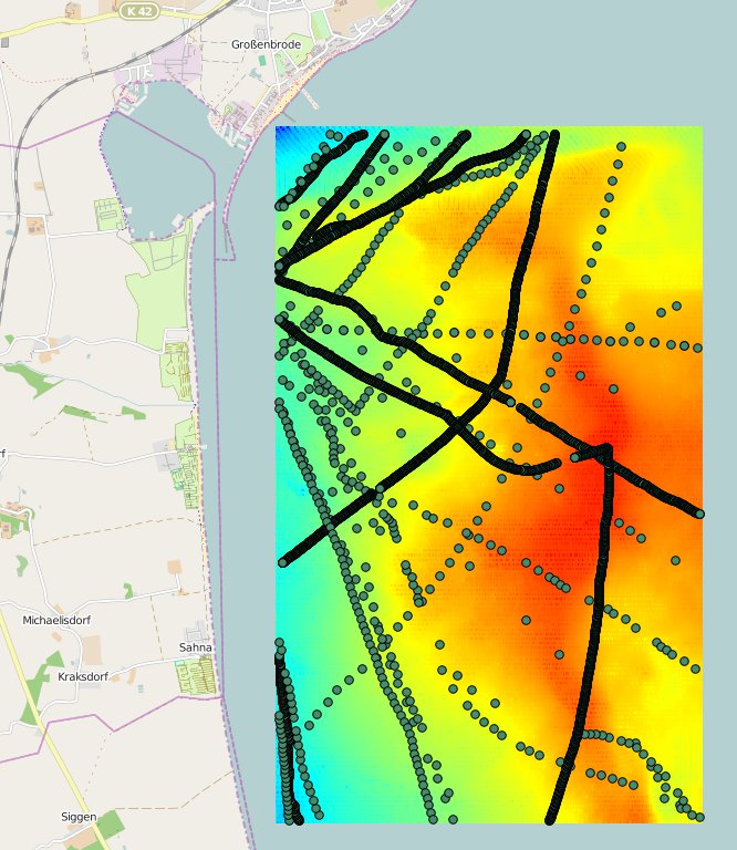
Baltic Sea - near Großenbrode (Germany)
First results with an RMS error < 1,5 meter compared to an official dataset of the Bundesamt für Seeschifffahrt und Hydrographie (BSH) [1].
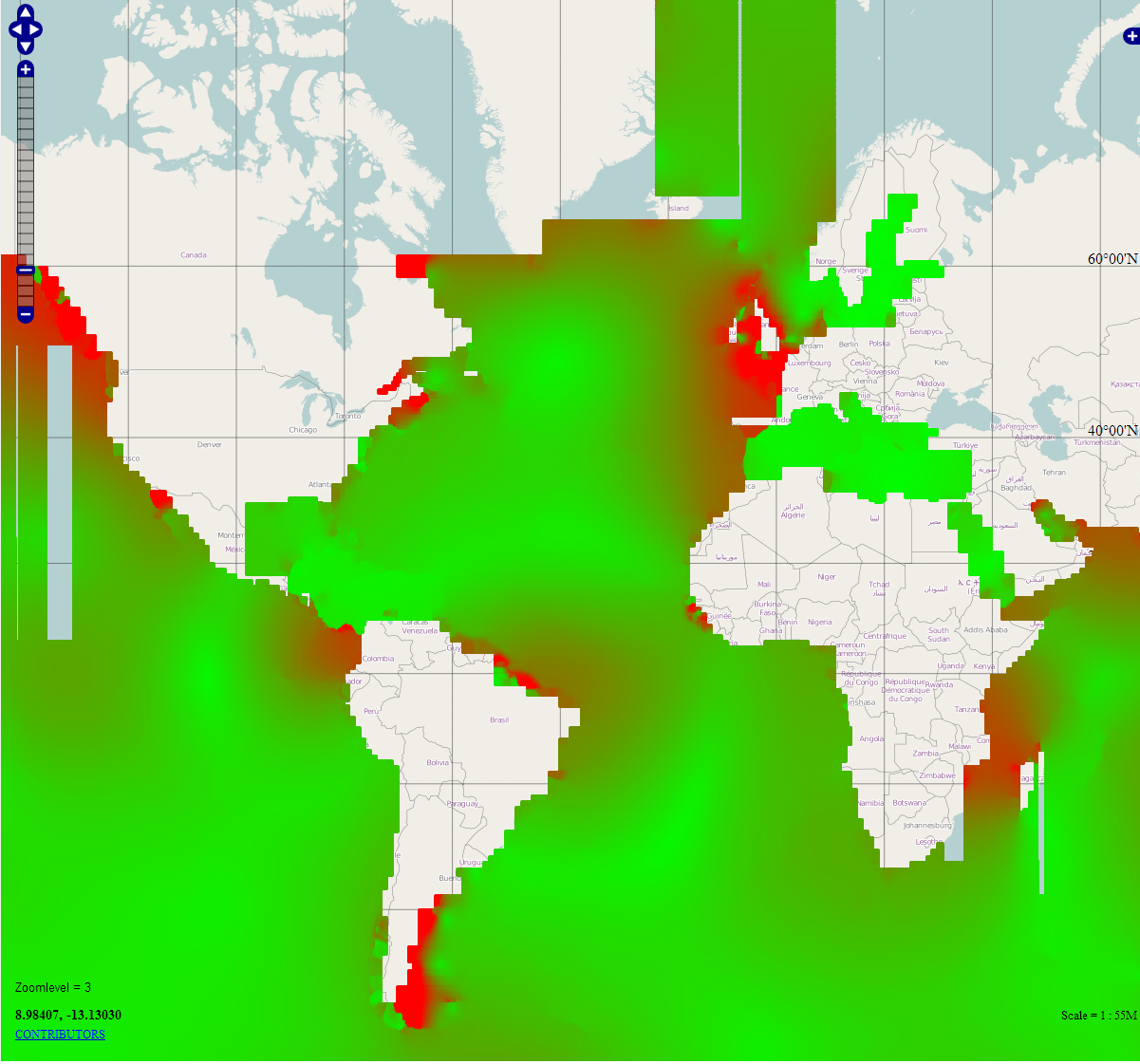
[Picture 1] OSM map in background, raster Depth Model derived from BSH data and crowed sourced OpenSeaMap Points - Overview
Blue = flat BSH data, red = deep BSH data.
Blue points = OpenSeaMap raw measuring points.
| n | 5062 |
| datasets | 21 |
| max deviation | 3,43 meters |
| mean (abs) | 0,69 meters |
| RMS +/- | 0,91 meters |
Vessel Metadata
| VesselConfig ID | 68 |
| Manufacturer | Bavaria Yachtbau |
| Model | B32 |
| Length | 10,0 meters |
| Beam | 3,35 meters |
| Draft | 1,6 meters |
| Height | 14 meters |
| Displacement | 4,2 t |
| Sensor manufacturer | Raymarine |
| Sensor Offset to waterline | 0,45 meters |
| Sensor Offset to keel | 1,15 meters |
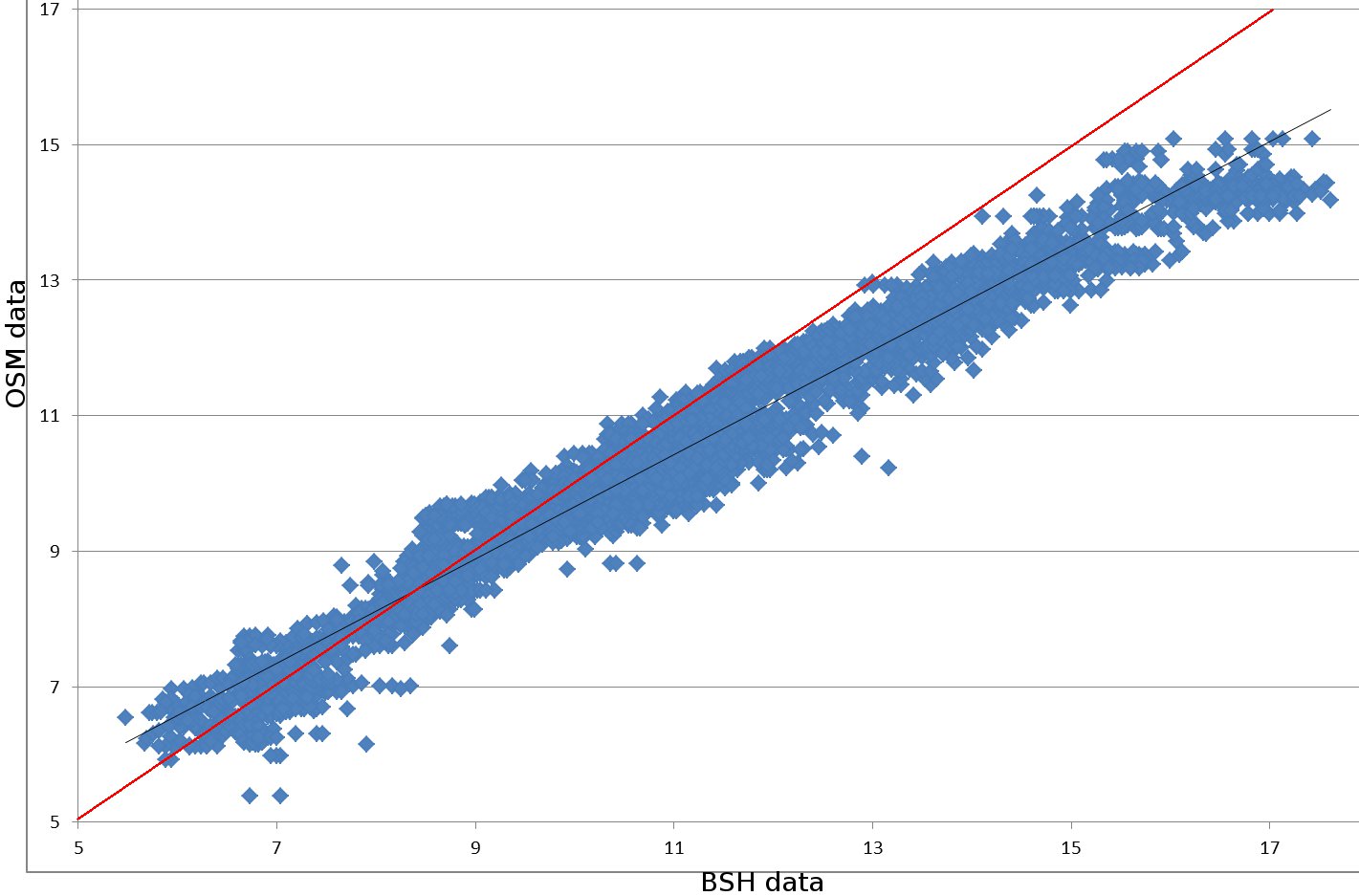
A digital Deep Model raster was computed from the BSH point dataset (c). The depth of the crowed sourced dataset was compared to the derived raster dataset from the BSH. The raw crowed sourced dataset was corrected by the sensor offset (0,45 meters).
[Picture 2] Scatter plot: BSH data on the x-axis and the crowed sourced data on the y-axis. Trend line in black and optimal line in red.
The deviation from the reference dataset increases with the depth measured.
As you see in the picture below the difference between the datasets has an regular pattern maybe deepending on waves.
[Picture 3] Crowed sourced OpenSeaMap track points and the difference from the BSH dataset
White = low difference, orange = medium difference, red = strong difference
Download of the data http://osm.franken.de/data/baltic_sea_test_data.zip Be aware of the copyright from the Bundesamt für Seeschifffahrt und Hydrographie (BSH) [2]. The data in the dataset is not corrected by sensor offset.
Baltic Sea Olpenitz (Germany)
In this test area we have tracks from two different vessel configurations. The fist one was the one from the test area Großenbrode (config ID 68).
In the Table below the settings for die vesselconfigid 110 are shown:
Vessel Metadata
| VesselConfigId | 110 |
| Manufacturer | Waarschip |
| Model | 570 |
| Length | 5,7 meters |
| Beam | 2,45 meters |
| Draft | 1,0 meters |
| Height | 9.1 meters |
| Displacement | 0,8 t |
| Sensor manufacturer | Tacktick/ Airmar |
| Sensor Model | T912 |
| Sensor Offset to waterline | 0,2 meters |
| Sensor Offset to keel | 0,45 meters |
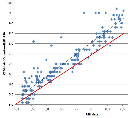
[Picture 1] Scatterplot for vesselconfigID 110. Trendline in Black and optimal line in red (after correction of the sensor offset to waterline).
| vsselConfigId | 110 |
| n | 247 |
| mean | 0,49 meters |
| rms | 0,62 meters |
| max | 2,53 meters |
The distribution is quite different from the data recorded in the test area Großenbrode with an different sensor.
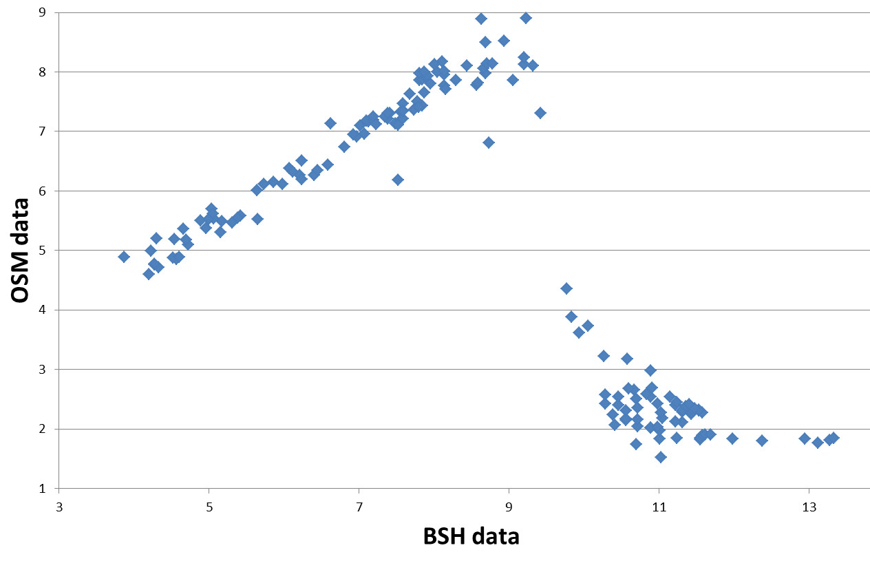
Fortunately we have also data from the VesselConfigId 68 in this test area to compare the measurements.
[Picture 2] Scatterplot for vesselconfigID 68 after correction of the sensor offset to waterline.
Obviously there are some outliers which are shown in picture 3.
[Picture 2] Outliers along the track 9064 in yellow - vesselconfigID 68.
Without the outliers the behavier of distribution is very same the results in the test area Großenbrode.
[Picture 1] Scatterplot for vesselconfigID 68 without outliers. Trendline in Black and optimal line in red (after correction of the sensor offset to waterline).
| vsselConfigId | 68 () without outliers |
| n | 100 |
| mean | 0,38 meters |
| rms | 0,53 meters |
| max | 2,1 meters |
Preliminary Conclusions
1. The distribution of the data derived from the measurements depends on the sensor. The realationships are almost linear and could be corrected if the sensor is known. Therefore the fill out in the form of the Web Frontend should be obligatory.
2. The sensor offset to the waterline is very easy to correct and should be obligatory in the fill out in the form.
3. There are outliers which should be investigated. Perhaps this data could be corrected or identified with the data from the uploaded tracks (speed, etc.).
Meta Data Statistics
Statistics for the metadata entrees with some personal comments (by MartinOver). Stand 20.9.2014.
|
Step |
Topic |
Count |
State |
Comment |
|
1/1 |
Name |
118/118 |
Obligatory |
|
|
1/2 |
Description |
76/118 |
Manditory |
|
|
2/1 |
Length |
60/118 |
Obligatory |
Some wrong entrees like mail addresses or comments 24 “0.00” Values |
|
2/2 |
Beam |
118/118 |
Obligatory |
37 „0.00“ Values |
|
2/3 |
Draft |
79/118 |
Manditory |
|
|
2/4 |
Displacement |
72/118 |
Manditory |
|
|
2/5 |
Height |
78/118 |
Manditory |
|
|
2/6 |
Manufacturer |
52/118 |
Manditory |
|
|
2/7 |
Model |
49/118 |
Manditory |
|
|
2/7 |
Type |
72/118 |
Manditory |
|
|
3/1 |
Distance from Stern |
118/118 |
Obligatory |
55 “0.0” Values |
|
3/2 |
Distance from Centerline |
118/118 |
Obligatory |
55 “0.0” Values |
|
3/3 |
Position below Waterline |
57/118 |
Manditory |
Should be Obligatory |
|
3/4 |
Depth Measurement |
? |
Manditory |
Where in DB? |
|
3/5 |
Sensor Offset to Keel |
6/118 |
Manditory |
|
|
3/6 |
Producer of Depth Sensor |
63/118 |
Manditory |
|
|
3/7 |
Device Model |
40/118 |
Manditory |
|
|
4/1 |
Distance from Stern |
118/118 |
Obligatory |
58 „0.0“ Values |
|
4/2 |
Distance from Centerline |
118/118 |
Obligatory |
51 „0.0“ Values |
|
4/3 |
Position abbove Waterline |
52/118 |
Manditory |
|
|
4/4 |
Producer |
77/118 |
Manditory |
|
|
4/5 |
Model |
60/118 |
Manditory |
|
Data Preprocessing
Data Condition
Raw data is usually erronous and must be corrected
Internal data problems
Depth data may be affected by electrical conditions and software implementations
- Data is incomplete and fail their checksum (bus errors from physical transmissions errors)
- Data is retrived out of sequence
- Data is erronous sensor data
- Approximate correctable data i.e. invalid GPS position that may be interpolated
- Uncorrectable data i.e. failed log sensor that shows slow speeds
- Data resolution is low i.e. for energy saving purposes GPS position is updated every 10 seconds instead of every second
- Sensor data is actively miscalibrated i.e. charter companies add additional draft to the sensor depth for safety reasons
External data problems
Depth data may be affected by different environmental circumstances
- The water temperature affects the ultrasound echo. An inhomogen water temperature yields unwanted echos
- The seabed affects the ultrasound echo
- The seastate affects the measurement. There even may be waves when there is no wind.
- Waves may affect the roll of the measuring vessel resulting in steep measurements that are invalid.
- The sounder sensor is not the position of the GPS antenna. A position offset including heading must be incorporated.
- The time of the measurement need not correlate with the time the position was received. This may even happen due to processing time of the hard or software.
- Corrections for tide induced water levels must happen
Solutions probably are
- Water temperature may be measure from the sensor, other data may be unavailable
- Modern sidescan sonar may yield information about the seabed through classifications
- A gyro and accelerometer may be used to remove the waves
- A gyro and accelerometer may be used to remove the waves
- Position offsets must be provided by the user
- Time outages may be handled by the filter if precise timestamps are available in recorded data
- LAT to Mean sea level differences may be calculated from DTU10 worldwide, river gauges need to monitored
Data Condition Examples / Showcases
Missing measurments (Position)
Distribution for position updates taken from an example dataset. Left column shows the time between two consecutive measurements, right column shows how many measurements had this time update. One can see from the distribtion that the sensor is updated every second but many measurements are one or more seconds late. 21 seconds with no position update may result in an instability of the subsequent filter.
MeasuredPosition3D
	GP
		0	:4285
		1000	:11295
		2000	:5056
		3000	:2134
		4000	:1135
		5000	:315
		6000	:154
		7000	:46
		8000	:36
		9000	:16
		10000	:12
		11000	:3
		12000	:4
		13000	:1
		14000	:7
		15000	:3
		16000	:1
		21000	:1
Missing measurments (Position) with erronous clock
This example is at a 10 second position update rate. However the measurment time is faulty causing large negative and positive update rates. The clock jumps by +- one year/month/day/hour. One can further see from the many 0 time measurements that the rate at which data is sent to the nmea bus is higher than the actual position update (data is sent every second, a position update is every 10 seconds)
MeasuredPosition3D
	II
		-21340000	:1
		-13194000	:1
		-7998000	:1
		-2674000	:1
		-2434000	:1
		-2402000	:1
		-2030000	:1
		-1926000	:1
		-1894000	:1
		-1806000	:1
		-1480000	:1
		-1430000	:1
		-1382000	:1
		-1114000	:1
		-814000	:1
		-634000	:1
		-590000	:1
		-546000	:1
		-470000	:1
		-290000	:1
		-230000	:1
		-198000	:1
		-110000	:1
		-94000	:2
		0	:182200
		5000	:1
		10000	:20230
		15000	:1
		20000	:84
		50000	:1
		114000	:2
		130000	:2
		218000	:1
		250000	:1
		310000	:1
		490000	:1
		566000	:1
		610000	:1
		654000	:1
		834000	:1
		1134000	:1
		1402000	:1
		1450000	:1
Solution Proposal
Outline
The ship is influenced by the outlined environment which can be observed. Naturally what is observed is not the state of the ship as i.e. the position if taken from GPS is 95% less than 10m accurate. To improve quality an estimation of the true state yields better results if this noise taken into account properly.
Details
The ship moves according to physical laws. For the easist case imagine a ship with constant velocity and direction. For any point in time you can tell where the ship is with easy math. Considering the full blown setup a ships movement is affected by many parameters such as wind speed, water current, waves, tide, and many more. The ship moves also triaxial in a dynamic way in itself (roll, pitch, yaw). Heeling even changes the measurement position with respect to the depth position. In terms of a filter this is called a system model that describes how the state of the ship may change. Given such a state you can measure what your sensor readings are and compare that to where the system thinks you are.
The Kalman Filter is known to be the best linear estimator for such situations. Unfortunately the system model is not linear which is why the Extended Kalman Filter needs to be used in order to linearize the system at hand.
Todo:
- Construct ship system model with at least the position state and probably its course and speed or even more (depth)
- Estimate the system variance (This is a hard one, proposals welcome)
- Construct the measurement model according to the data available (GPS, Log)
- Estimate the measurement noise according to specifc sensors (DPGS is more accurate than GPS)
The estimation with the position and depth can be retrieved and stored in a database.
Pitfalls:
- If the system noise is badly chosen the estimation of the system state does not converge to the true state / measurement.
- If the system is very detailed the system variance can be reduced. The required cpu time for processing increases
Benefits:
- Having the best estimation of the true position even if measurements are noisy
- Easy and effective algorithmic processing
Analysis
Data Sets
Currently two test data sets are available recorded during trips from Mallorca and the Baltic Sea. In terms of data quality the Mallorca data shows many challenges.
- The minimum recommended sentences from NMEA showed up with false date and time readings while having correct (!!!) message checksums.
- The log on the ship was defective and delivered no readings from time to time.
- The same holds true for the water temperature.
- The GPS positions relatively imprecise because some last decimal digits are missing in the recordings.
- The GPS positions are updated every 10 seconds while other sensor readings update almost every second.
- The GPS position are sometimes way off due to false readings
The Baltic Sea data set is a little bit better
- Only a single day is available
- GPS positions are updated every second
One problem with the data is that there is time available when sensor readings were recorded. This yields problems to the filter algorithm.
Filter Algorithm
At first the Extended Kalman Filter is being analyzed. Using an apache implementation with the available data the filter quickly throw an exception that a matrix is not invertible because of numeric instabilities. When removing this exception the filter seems to work but the removal and its effects have yet to be analyzed. Literature suggest that a fixed interval smoother may yield better results in case of offline data processing. As it is an extension to the existing kalman filter we may consider that for the future.
One problem are the different update rates of the sensors. As GPS may deliver positions at 0.1Hz speed is updated at 1Hz. Literature suggests that the missing measurements shell be modelled as a random variable with the standard deviation of the sensor. It may even be possible to update covariance matrices only partially with the sensor readings received. Input for the best solution may be formulated on the developer mailing list.
Results
A prototype implementation is shown in the following screenshots. An Extended Kalman Filter is being used. It has the position and the current bearing and velocity as system state. The input is the measurement of these four observables. The system function is good old pythagoras. In a first implementation I tried to use orthodrome distances but the system function is not differentiable which is a requirement of the Extended Kalman Filter (due to acrtan2). For small distances pythagoras should be sufficiently accurate. The initial state is taken from the first measurement for convergence reasons.
The following gallery shows the results.
- You can see the bad position resolution and an outlier in the first screenshot.
- The second shows the same data overlaid with the applied filter. The outlier is gone and the resolution has improved.
- The third screenshot shows data from a different GPS sensor with more precision (not DGPS) versus the filtered data.
This of course is just a preliminary test and many setups need to be considered to make it work for most datasets.
The overall process even gives an estimation of the current error which is a capability of the Kalman Filter. This way positional inaccuracies may be added to the overall depth measurement inaccuracy.
Quality rating
Each record (time, positon, depth) should become a quality rating.
Points
Derived from the Fibonacci series.
| Point | Description |
|---|---|
| 1 | extra small improvement |
| 2 | small improvement |
| 3 | medium improvement |
| 5 | large improvement |
| 8 | extra large improvement |
Factors
| Name | Factor | Description |
|---|---|---|
| depth offset | 8 (extra large) | The difference between the depth measured by the echo sounder and the depth (waterline) measured by hand. |
| device distance | 3 (medium) | The distance between gps antenna and echo sounder (lengthwise and crosswise). |
| SBAS | 3 (medium) | Satellite based augmentation system (WAAS, EGNOS, MSAS) which allows to correct the gps position. |
| position interpolation | 2 (small improvement) | Arrival of depth and position packets can have a time difference. It is/should be possible to interpolate the position. |

